Activation Functions and Their Gradients
Activation functions are the last step in an artificial neuron's activity, and it is from these functions that artificial neural networks can learn to express nonlinear functions. All these functions do is map the "hidden" value of a neuron to the output, so for a single artificial neuron, they map:
$f: \mathbb{R} \rightarrow \mathbb{R}$
However, since we can express Artificial Neural Networks as linear algebra where weights and biases are matrices and vectors, we instead consider an activation function to be constant across a layer, and therefore applied to each "hidden" value of each artificial neuron in that layer. We instead apply an activation function to a vector, which maps:
$f: \mathbb{R}^i \rightarrow \mathbb{R}^o$
where $i$ is the dimension of the input vector, and $o$ is the dimension of the output vector. When we use these functions to implement a layer in an artificial neural network, we will, for activation function $f$, compute:
$A = f(\textbf{X}\cdot\textbf{W}+\textbf{b})$
Where $\textbf{X}$ is the input to a layer, $\textbf{W}$ and $\textbf{b}$ are the parameters of the layer. From here, we can further subdivide activation functions into two types: $\textbf{element-wise independent functions}$ and $\textbf{element-wise dependent functions}$ that have different properties. Below we will cover some popular activation functions, their gradients, and their numpy implementations.
Element-wise Independent Functions
Element-wise Independent functions are applied independently to each element of the input vector. More specifically, if we have a function $f$ and a vector $\textbf{x} = \{x_1, x_2, \dots, x_n\}$, we compute $f(\textbf{x}) = \{f(x_1), f(x_2), \dots, f(x_n)\}$. This matters when computing the gradient of our activation function with respect to an input vector $\textbf{x}$. So how do we compute gradients of element-wise independent activation functions? Well, technically we need to compute a Jacobian matrix that computes the partial derivative of each input variable to each output variable. For an input vector $\textbf{x} = \{x_1, x_2, \dots, x_n\}$ and output vector $f(\textbf{a}) = \{a_1, a_2, \dots, a_n\}$, the Jacobian $\textbf{J}$ will be an $n \times n$ matrix and look like:
$$J = \begin{bmatrix} \frac{\partial a_{1}}{\partial x_{1}} & \frac{\partial a_{2}}{\partial x_{1}} & \dots & \frac{\partial a_{n}}{\partial x_{1}} \\ \frac{\partial a_{1}}{\partial x_{2}} & \frac{\partial a_{2}}{\partial x_{2}} & \dots & \frac{\partial a_{n}}{\partial x_{2}} \\ \vdots & \vdots & \ddots & \vdots \\ \frac{\partial a_{1}}{\partial x_{n}} & \frac{\partial a_{2}}{\partial x_{n}} & \dots & \frac{\partial a_{n}}{\partial x_{n}} \\ \end{bmatrix}$$The reason we separate element-wise independent from element-wise dependent functions is because of a significant optimization we can make for this Jacobian. Since we are talking about element-wise $\textit{independent}$ functions, we know that $a_i$ is only dependent on $x_i$ since $a_i = f(x_i)$ and independent of all other elements of the input vector $\textbf{x}$. Therefore, any term $\frac{\partial a_i}{\partial x_j}$ where $i \ne j$ is 0. Our Jacobian is $\textit{sparse}$, specifically the diagonal of $\textbf{J}$ are the only terms that can be nonzero:
$$J = \begin{bmatrix} \frac{\partial a_{1}}{\partial x_{1}} & 0 & \dots & 0 \\ 0 & \frac{\partial a_{2}}{\partial x_{2}} & \dots & 0 \\ \vdots & \vdots & \ddots & \vdots \\ 0 & 0 & \dots & \frac{\partial a_{n}}{\partial x_{n}} \\ \end{bmatrix}$$The reason this is a huge optimization is because of how we are going to use this Jacobian matrix. We want to compute the three gradients of a layer: $\frac{\partial f(\textbf{X}\cdot \textbf{W} + \textbf{b})}{\partial \textbf{X}}, \frac{\partial f(\textbf{X}\cdot \textbf{W} + \textbf{b})}{\partial \textbf{W}},$ and $\frac{\partial f(\textbf{X}\cdot \textbf{W} + \textbf{b})}{\partial \textbf{b}}$. We can use the chain rule here to rewrite some terms and make it easier to deal with:
$$\begin{eqnarray} Z &=& \textbf{X}\cdot\textbf{W}+\textbf{b}\\ A &=& f(\textbf{Z}) \end{eqnarray}$$Ok, so now what we are looking for are the three gradients:
$$\begin{eqnarray} \frac{\partial f(\textbf{Z})}{\partial \textbf{X}} &=& \frac{\partial f(\textbf{Z})}{\partial \textbf{Z}}\frac{\partial \textbf{Z}}{\partial \textbf{X}} &=& \textbf{J}\frac{\partial \textbf{Z}}{\partial \textbf{X}}\\ \frac{\partial f(\textbf{Z})}{\partial \textbf{W}} &=& \frac{\partial f(\textbf{Z})}{\partial \textbf{Z}}\frac{\partial \textbf{Z}}{\partial \textbf{W}} &=& \textbf{J}\frac{\partial \textbf{Z}}{\partial \textbf{W}}\\ \frac{\partial f(\textbf{Z})}{\partial \textbf{b}} &=& \frac{\partial f(\textbf{Z})}{\partial \textbf{Z}}\frac{\partial \textbf{Z}}{\partial \textbf{b}} &=& \textbf{J}\frac{\partial \textbf{Z}}{\partial \textbf{b}} \end{eqnarray}$$So we see that we will have to be using some matrix multiplication here. We can reduce this matrix multiplication down to element-wise multiplication if we know that $\textbf{J}$ is sparse and only contains a gradient along the diagonal. This optimization will save us tons of time, especially as the parameter space and feature space of our models grow.
Lets define some popular element-wise independent functions and show their numpy implementations. Since these are element-wise independent functions, when we define them, we will talk about them given scalar inputs instead of vector inputs. Just remember that when we apply these to vectors, we apply the function to each element of the input vector.
Sigmoid
The sigmoid activation function is perhaps the most popular one of them all. Sigmoid is defined as:
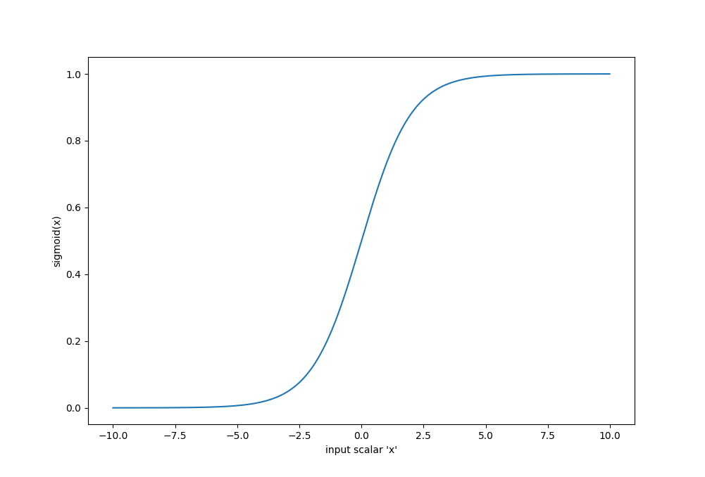 $$\sigma(x) = \frac{1}{1+e^{-x}}$$
Sigmoid has a range of [0, 1], and a picture of its shape is on the right. Sigmoid comes from the "step-function" assumption that real neurons were theorized to have back in the 1970s, the real only difference being that this function is smooth and differentiable. Remember, artificial neural networks are trained by computing gradients, and therefore require all all components to be differentiable.
What is the gradient of the sigmoid function? Well, we'll only cover the gradient only along the diagonal of the Jacobian, so we only need to worry about the derivative of each vector element individually, and therefore we can express this as the $\textit{derivative}$ of sigmoid instead of a partial derivative:
$$\begin{eqnarray} \frac{d \sigma(x)}{dx} &=& \frac{d \frac{1}{1+e^{-x}}}{dx}\\ &=& \frac{(1+e^{-x})*\frac{d 1}{dx} - 1*\frac{d (1+e^{-x})}{dx}}{(1+e^{-x})^2}\\ &=& \frac{e^{-x}}{(1+e^{-x})^2}\\ &=& \frac{1+e^{-x}-1}{(1+e^{-x})^2}\\ &=& \frac{1}{1+e^{-x}}-\frac{1}{(1+e^{-x})^2}\\ &=& \sigma(x) - (\sigma(x))^2\\ &=& \sigma(x)(1-\sigma(x)) \end{eqnarray}$$Note: it is quite common for the gradient of an activation function to be expressable in terms of the activation function itself. Alright, lets talk about how we would implement an arbitrary activation function in numpy. I kind of like the idea of allowing people to pass in references to their activation functions, rather than specify them by string values and a lookup table. So, to minimize the amount of parameters needed (remember, we need to keep track of two references per activation function: the function itself, and the function that computes it's gradient), I am going to implement activation functions as $\textit{functors}$. A Functor is an object that "pretends" to be a function (i.e. is callable). In Python, to make an object callable, all we need to do is override the __call__ method. By making each activation function a functor, we can create two methods: one to call the function, and another to compute the gradient. Here is what the sigmoid object will look like:
                class Sigmoid(object):
                    def __init__(self):
                        pass

                    def __call__(self, X):
                        return 1.0/(1.0+np.exp(-X))

                    def gradient(self, X):
                        Q = self(X)
                        return Q*(1-Q)
Tanh
Tanh is another popular activation function, and while it has a similar shape to sigmoid, it has a different range, and a different gradient. Tanh is defined as:
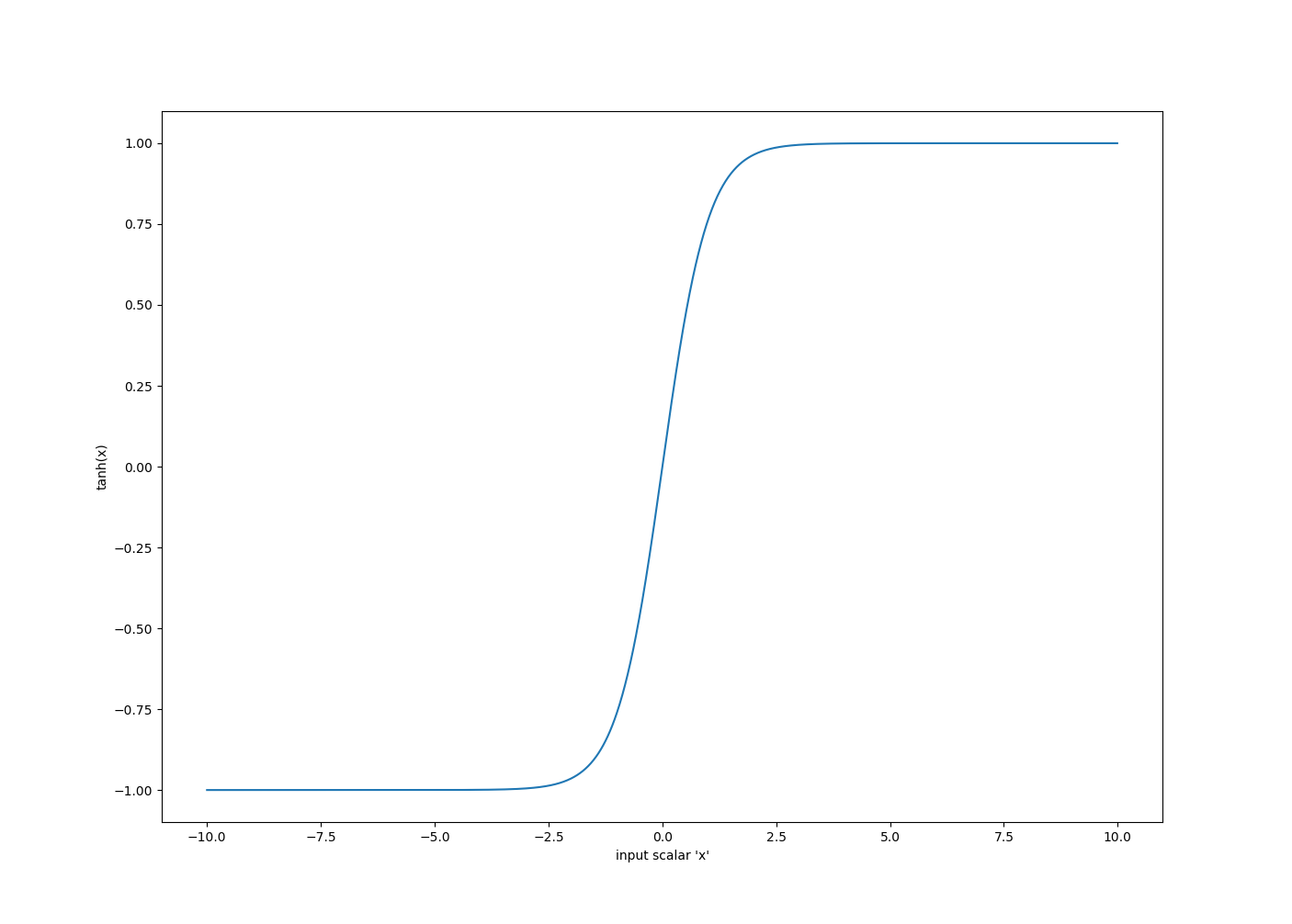 $$tanh(x) = \frac{sinh(x)}{cosh(x)} = \frac{e^{x}-e^{-x}}{e^{x}+e^{-x}}$$
Its gradient, just like sigmoid, can be expressed as the derivative of each element:
$$\begin{eqnarray} \frac{d tanh(x)}{dx} &=& \frac{d \frac{sinh(x)}{cosh(x)}}{dx}\\ &=& \frac{cosh(x)\frac{d sinh(x)}{dx}-sinh(x)\frac{d cosh(x)}{dx}}{(cosh(x))^2}\\ &=& \frac{(cosh(x))^2-(sinh(x))^2}{(cosh(x))^2}\\ &=& 1-(\frac{sinh(x)}{cosh(x)})^2\\ &=& 1-(tanh(x))^2 \end{eqnarray}$$Following our functor structure, we can implement tanh like:
                class Tanh(object):
                    def __init__(self):
                        pass

                    def __call__(self, X):
                        return np.tanh(X)

                    def gradient(self, X):
                        return 1-np.tanh(X)**2
Linear
One of the most overlooked and least interesting activation functions is the linear function. Personally, I hate this name, because the linear activation function returns the input value, so I think it should be called the identity activation:
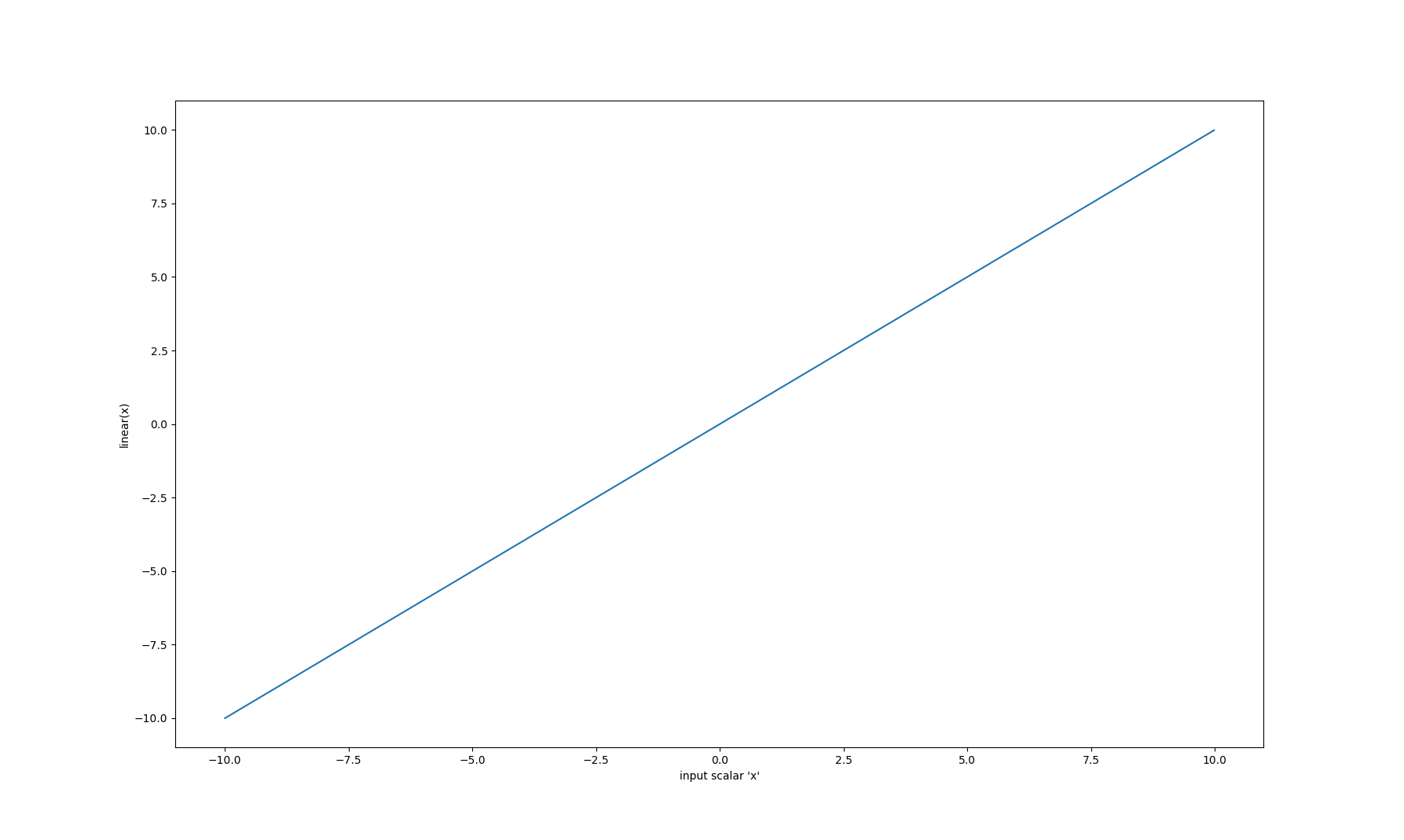 $$f(x) = x$$
This activation function serves the same purpose as not having one at all. Why does it exist? Typically, most implementations require you to specify an activation function, so this serves as the "filler" role. Its gradient is extremely uninteresting:
$$\begin{eqnarray} \frac{d f(x)}{dx} &=& \frac{dx}{dx} = 1 \end{eqnarray}$$As a functor:
                class Linear(object):
                    def __init__(self):
                        pass

                    def __call__(self, X):
                        return X

                    def gradient(self, X):
                        return np.ones(X.shape, dtype=float)
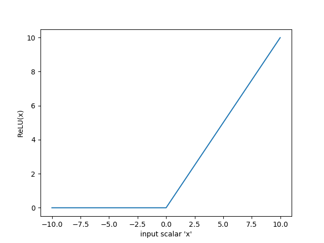
ReLU
The REctified Linear Unit is one of the most interesting functions in this list. ReLU is the first (and only) piecewise function we will discuss. The idea is that we don't want negative activations, and also don't want to force activations between a range (like tanh or sigmoid). Therefore, ReLU is piecewise defined as:
 $$ReLU(x) = \begin{cases}
x & x \ge 0\\
0 & otherwise
\end{cases}$$
$$ReLU(x) = \begin{cases}
x & x \ge 0\\
0 & otherwise
\end{cases}$$
Interestingly, ReLU is one of the most successful activation functions: models that use ReLU activations often learn much quicker than the same model does without using ReLU activations. Just as ReLU is piecewise defined, it also has a piecewise derivative:
$$\begin{eqnarray} \frac{d ReLU(x)}{dx} &=& \begin{cases} \frac{dx}{dx} & x \ge 0\\ \frac{d0}{dx} & otherwise \end{cases}\\ &=& \begin{cases} 1 & x \ge 0\\ 0 & otherwise \end{cases} \end{eqnarray}$$One point to mention is that $\frac{d ReLU(x)}{dx}$ does not exist when $x == 0$. One solution to this (that we will use), is to arbitrarily choose a value for the derivative when $x == 0$. Personally, I choose the value 1, because according to the piecewise definition, when x is 0, if we decided to return x (ReLU(x) = x), then the derivative would be 1. Common values are 0, 0.5, or 1. Another common solution is to use an approximate ReLU function that is differentiable for all x. Such a function could be:
$$f(x) = ln(1+e^{x})$$which has derivative:
$$\begin{eqnarray} \frac{df(x)}{dx} &=& \frac{e^{x}}{1+e^{x}}(\frac{\frac{1}{e^{x}}}{\frac{1}{e^{x}}})\\ &=& \frac{1}{1+e^{-x}}\\ &=& \sigma(x) \end{eqnarray}$$ReLU is also extremely easy to implement:
                class ReLU(object):
                    def __init__(self):
                        pass

                    def __call__(self, X):
                        Y = np.zeros(X.shape, dtype=float)
                        Y[X>0] = X[X>0]
                        return Y

                    def gradient(self, X):
                        Y = self(X)
                        Y[Y>=0] = 1 # note I am considering df/dx @ x=0 to be 1
                        return Y
Element-wise Dependent Functions
Element-wise dependent functions consist of the class of functions where each value in an output vector $\textbf{a} = \{a_1, a_2, \dots, a_n\}$ is a function of multiple values in the input vector $\textbf{x} = \{x_1, x_2, \dots, x_n\}$. Sadly, with this class of functions, the Jacobian $\textbf{J}$ is not a diagonal matrix, and we have to perform the full matrix multiplication instead of element-wise multiplication optimization. There are only a few element-wise dependent activation functions, but we are only going to cover the most popular.
Softmax
Softmax is one of the most important activation functions out there. We will start with the definition, and then explain why:
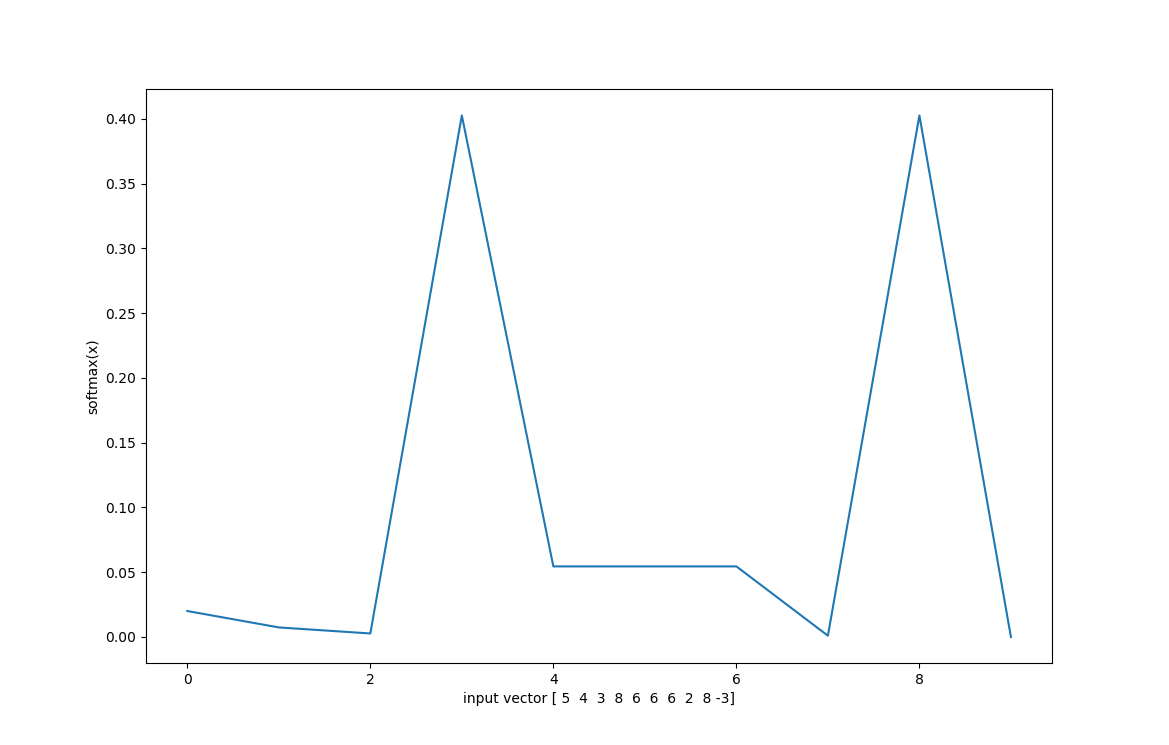 $$softmax(\textbf{x}) = \{\frac{e^{sx_1}}{\sum\limits_{k=1}^{n} e^{sx_k}}, \frac{e^{sx_2}}{\sum\limits_{k=1}^{n} e^{sx_k}}, \dots, \frac{e^{sx_n}}{\sum\limits_{k=1}^{n} e^{sx_k}}\}$$
Ok, theres a lot to unpack here. $softmax(\textbf{x})$ is only defined for vector operations, it cannot take a scalar input. $Softmax(\textbf{x})$ converts an input vector $\textbf{x}$ with $n$ elements into a probability distribution with $n$ elements. By exponentiating each term in the input vector, $softmax$ guarantees each term to be postive. By summing all exponentiated elements and dividing by that sum, $softmax$ computes a probability distribution by assigning each element in the output vector to be the percentage that the input element contributed to the sum. The variable $s$ is just a stretch parameter, it controls the variance of the distribution, or how "spread out" the distribution is.
One important thing to note here is that these probabilities are $\textbf{not}$ confidence values. If the value at position 1 in the output distribution is 0.95, that does $\textbf{not}$ mean that the model is 95% confident in its choice. We will cover why later when talk about thinking Bayesian, but the short answer is that there is that $softmax$ gives a probability distribution according to a single combination of parameters, to measure true confidence, we would need to consider the distribution of parameters. Again, more on this later.
Since $softmax$ is not element-wise independent, we need to compute each element of the Jacobian matrix $\textbf{J}$. Therefore, let us compute start with the formula for an individual element of $\textbf{J}$ (output position $i$ and input position $j$):
$$\begin{eqnarray} \frac{d softmax_i(\textbf{x})}{dx_j} &=& \frac{d\frac{e^{sx_i}}{\sum\limits_{k=1}^{n} e^{sx_k}}}{dx_j}\\ &=& \frac{(\sum\limits_{k=1}^{n} e^{sx_k})\frac{d e^{sx_i}}{dx_j} - e^{sx_i}\frac{d\sum\limits_{k=1}^{n} e^{sx_k}}{dx_j}}{(\sum\limits_{k=1}^{n} e^{sx_k})^2}\\ &=& \frac{\frac{de^{sx_i}}{dx_j}}{\sum\limits_{k=1}^{n} e^{sx_k}} - \frac{e^{sx_i}se^{sx_j}}{(\sum\limits_{k=1}^{n} e^{sx_k})^2} \end{eqnarray}$$This is a far as we can go without knowing the relationship between $i$ and $j$. If $i == j$, then:
$$\begin{eqnarray} &=& \frac{se^{sx_j}}{\sum\limits_{k=1}^{n} e^{sx_k}} - s(\frac{e^{sx_j}}{\sum\limits_{k=1}^{n} e^{sx_k}})^2\\ &=& s*softmax_i(\textbf{x})*(1-softmax_i(\textbf{x})) \end{eqnarray}$$If $i \ne j$:
$$\begin{eqnarray} &=& 0 - s\frac{e^{sx_i}e^{sx_j}}{(\sum\limits_{k=1}^{n} e^{sx_k})^2}\\ &=& s*softmax_i(\textbf{x})*softmax_j(\textbf{x}) \end{eqnarray}$$We can combine these two expressions to form a piecewise expression:
$$\frac{d softmax_i(\textbf{x})}{dx_j} = \begin{cases} s*softmax_i(\textbf{x})*(1-softmax_i(\textbf{x})) & i==j\\ s*softmax_i(\textbf{x})*softmax_j(\textbf{x}) & otherwise \end{cases}$$This is annoying to keep track of, so mathematicians invented the Kronecker delta function. The Kronecker delta is a compact way of writing:
$$\delta_{ij} = \begin{cases} 1 & i==j\\ 0 & otherwise \end{cases}$$We can use the Kronecker delta to compress our $softmax$ gradient element:
$$\frac{d softmax_i(\textbf{x})}{dx_j} = s*softmax_i(\textbf{x})*(\delta_{ij}-softmax_j(\textbf{x}))$$Ok, now lets implement this. There are some implementation details worth mentioning. First, $softmax$ is not very numically stable for machines in its current formulation. This is because we risk overflow from really large values. So, one way to make this more numically stable is to subtract the max value of $\textbf{x}$ from each element in $\textbf{x}$. This subtraction will remove outlier values that might overflow, and $e^{x}$ where $x$ is a large negative number is stable. Additionally, if we keep this subtraction in the denominator, it will not affect the resulting probability distribution: $$\begin{eqnarray} softmax_i(\textbf{x}) &=& \frac{e^{s(x_i-max(\textbf{x}))}}{\sum\limits_{k=1}^{n} e^{s(x_k - max(\textbf{x}))}}\\ &=& \frac{e^{sx_i}e^{s*max(\textbf{x})}}{\sum\limits_{k=1}^{n} e^{sx_k}e^{s*max(\textbf{x})}}\\ &=& \frac{e^{sx_i}e^{s*max(\textbf{x})}}{e^{s*max(\textbf{x})} \sum\limits_{k=1}^{n} e^{sx_k}}\\ &=& \frac{e^{sx_i}}{\sum\limits_{k=1}^{n} e^{sx_k}} \end{eqnarray}$$
Which is the original formulation of $softmax$. Taking into account numerical stability, here is my functor:
                    class Softmax(object):
                        def __init__(self, stretch=1.0):
                            self.stretch = stretch

                        def __call__(self, X):
                            # This will only operate on the last axis
                            axis = -1
                            X_ = np.atleast_2d(X)*self.stretch
                            Y = np.exp(X_-np.expand_dims(np.max(X_, axis=axis), axis=axis))
                            Y /= np.expand_dims(np.sum(Y, axis=axis), axis=axis)

                            if len(X.shape) == 1:
                                Y = Y.flatten()
                            return Y

                        def single_jacobian(self, Y):
                            Y_ = Y.reshape(-1,1) # make 2D
                            return self.stretch*(np.diagflat(Y_)-np.dot(Y_, Y_.T))

                        def gradient(self, X):
                            Y = self(X)
                            out_shape = Y.shape + (Y.shape[-1],)
                            Y = np.atleast_2d(Y)

                            Y = Y.reshape(-1, Y.shape[-1])
                            out = np.zeros(Y.shape+(Y.shape[-1],), dtype=float)

                            # process each softmax vector
                            for i in range(Y.shape[0]):
                                out[i] = self.single_jacobian(Y[i])
                            return out.reshape(out_shape)

                            # interesting note here is that we could replace the python
                            # loop with a numpy C bound one. We could do it via the following:

                            # def f(a):
                            #     q = a.reshape(-1,1)
                            #     return np.dot(q, q.T)
                            # return (self.stretch*(np.apply_along_axis(np.diag,-1,Y)-np.apply_along_axis(f,-1,Y))).reshape(out_shape)

                            # one problem with this is that I measured it to be slower than
                            # the python loop! I think it has to do with np.apply_along_axis
                            # inferring the output shape rather than just assigning into
                            # a preallocated array with the python loop approach.
So at this point, our functors are also handling batch sizes, so the element-wise functors are expecting data with shape (batch_size, dim) and returning both gradients and outputs with the same shapes. Our $softmax$ functor will return outputs with the same shape as inputs, but will return a 3D matrix with shape (batch_size, dim, dim). To perform the matrix multiplication with a $softmax$ gradient, we will have to use the numpy expression
dLdSoftmax = np.einsum("...jk, ...kl", softmax_grad, np.expand_dims(dLdA_out, axis=-1), optimize=True).reshape(dLdA_out.shape)Now that we have activation functions out of the way, we can move on to defining loss functions and their gradients. I promise we'll get to the actual artificial neural networks soon!